Constrained data model - can you solve it?
By Murray Bourne, 21 Jul 2012
Constrained data model - can you solve it?
Statisticians are often asked to predict the future. Their job is to look at historical trends and to make their best guess what will happen tomorrow, or maybe next year. This involves a process called extrapolation, where we project into the future based on past data.
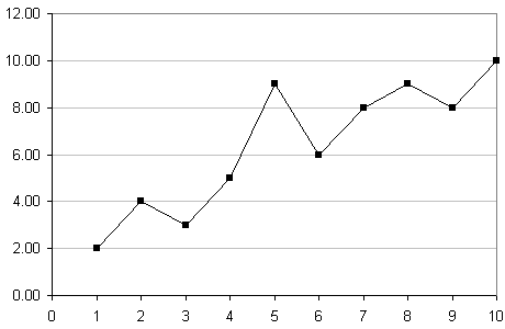
For example, here is a set of data representing company sales (variable s) for a period of 10 days (t):
| t | 1 | 2 | 3 | 4 | 5 | 6 | 7 | 8 | 9 | 10 |
|---|---|---|---|---|---|---|---|---|---|---|
| s | 2 | 4 | 3 | 5 | 9 | 6 | 8 | 9 | 8 | 10 |
Let's graph the data to get a better idea what it looks like:
To extrapolate intelligently, we need to consider the shape of the data curve, and then fit a curve as best we can through the points.
At the beginning, there is a steep rise in sales, but then it flattens out (perhaps the salespeople were getting tired). It appears to be a logarithmic curve, which in its standard form, starts fairly steeply, and then flattens out.
There are various formulas for fitting a curve to data (see the bottom of the page), but we'll use software.
We'll get Excel to draw a curve through the data points and then extrapolate for us. After entering the data in Excel, we highlight it, then choose the "XY(Scatter)" option. Once we see the chart, we select the graph and right click, then choose "Add trendline". We choose "logarithmic" because that's the shape of our data curve. Under "Options", we can choose to "Forecast" by as many steps as we like.
So in this next graph, you'll see the logarithmic growth model passing through the given data. I've forecast the next 20 days, so we can get an idea how our sales team will perform for the rest of the month, assuming their historical performance (for the first 10 days) continues.
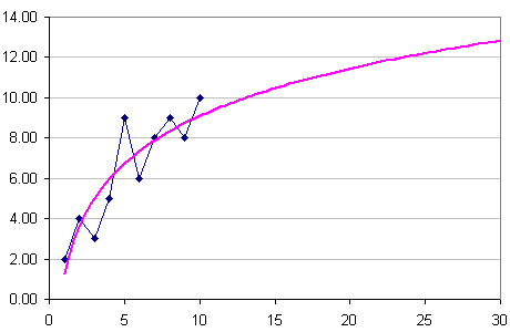
(The above set of data and curve is just to illustrate the problem. We need a formula that will work with any set of data, within the constraint mentioned next.)
Constraint
Now, (and here's where the challenge comes) say we need to produce a curve such that the sum of the values of the model curve is exactly the same as the sum of the values (for the first 10 days) in the original data set?
For example, here is the data again, but with a new row (m) containing values that fit the above constraint. That is, the sum of the first 10 sales values (variable s) is the same as the sum of the first 10 model values (using variable m).
| t | 1 | 2 | 3 | 4 | 5 | 6 | 7 | 8 | 9 | 10 | Σ |
|---|---|---|---|---|---|---|---|---|---|---|---|
| s | 2 | 4 | 3 | 5 | 9 | 6 | 8 | 9 | 8 | 10 | 64 |
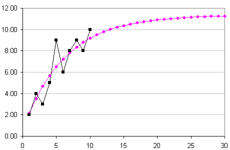
| m | 2.17 | 3.53 | 4.69 | 5.68 | 6.52 | 7.23 | 7.84 | 8.36 | 8.80 | 9.18 | 64 |
The sum (Σ) is given in the final column. Both rows s and m add to 64.
Here is the graph of the m-values given in the above table. You'll notice it is similar to the Excel logarithmic graph, but not exactly the same. I have once again extrapolated another 20 steps in the chart below. We observe using this constrained model that the sales per day at the end of the month is less (around 11.5) than Excel's logarithm curve (which gave almost 13).
So, your challenge is to develop a formula to produce a curve that goes through any set of data, given the above constraint. Good luck! (This is quite challenging, but give it a go.)
See the 10 Comments below.
25 Jul 2012 at 3:31 am [Comment permalink]
There is an underlying assumption concerning this problem that was not explicity stated: sales are reported as sales/salesperson. This cancels the effect of an expanding (or shrinking) sales force. Given that, the model suggests a logistic form. Why logistic? Presumably there is a learning curve for sales people to effectively promote a new product. Once they are proficient, there is a maximum number of sales that can be made per day (hours spent selling/time per sales pitch, assuming each sales pitch is successful!).
The logistic in its general form can be expressed as:
sales = A + (B - A)/(1 + (C/x)^D)
where
A = is the minimum number of sales per person per day
B = maximum number of sales per person per day
C,D determine slope and inflection point of the learning curve
This formula can be simplified by noting that A=0 (can't sell anything before you start).
I placed this equation and the data in Excel and used the equation solver as follows:
1. I defined the target cell as then squared error between the actual sales and predicted and minimized it.
2. Added the constraint that the sum of sales of the predicted had to equal the sum of sales of the raw data
3. Based on the original log-linear regression, I set the initial conditions as:
A=0
B=13.5
C=5
D=1
Furthermore, I instructed the solver to only alter parameters B and C, leaving A and D as specified. The resulting solution was:
A=0
B=15.2676679048944
C=6.63383395244721
D=1
The sum of the predicted sales was indeed 64, consistent with the stated constraint.
A plot of the predicted data closely matched your predicted values. The main difference is that at day 30, the logistic prediction was 12.5 sales vs your 11.5
I would be happy to provide the working spreadsheet on request.
Great question and challenge!
25 Jul 2012 at 8:59 am [Comment permalink]
Great solution, Peter. Your logistic equation makes a lot of sense, given the description of the problem.
I guess I should have said "keeping all other things equal" (so the sales force is the same throughout, their skill level is consistent and all those other unrealistic things that may or may not be going on in such a problem). However, my "sales" story and data was just to illustrate the kind of problem that we aim to model.
I realized after I posted the challenge that I hadn't explicitly stated that our formula must apply for any set of data. That is, we aim to find a model that will fit any shaped data while maintaining the constraint that the sum of the data values equals the sum of the model output values up to a known time value.
I amended the post to make that more clear. Very sorry to have led you up the garden path.
25 Jul 2012 at 1:26 pm [Comment permalink]
[...] squareCircleZ, Murray Bourne challenges you to predict the [...]
25 Jul 2012 at 4:25 pm [Comment permalink]
How about the following:
Let there be n data values, d(t), where t is time. Let the function you are fitting be f(a,t), where a is a vector of the constants to be found. Let g(f,a,t) be the function that represents the sum of f(a,t) over all the times for which you have data. Then minimise the differences between f(a,t)+w*(g(f,a,t) and d(t)+w*(sum of d(t)), using whatever is your favourite minimisation technique, where w is a weighting constant. Increase w until you are satisfied that the sum of the n fitted values adequately matches that of the data points.
Of course, the end result will still depend on the applicability of the form of function, f. In general, if the fitted function isn’t based on some underlying model, but just on guesswork, I’d be very wary of extrapolating.
30 Jul 2012 at 10:23 am [Comment permalink]
This may well drive me batty! I now understand that you wanted a generic solution, not one that depended on the logistic model, even thought that might make sense for this particular problem.
After plotting your predicted data against the logarithmic with a log scale along with the trending line, I noticed that the plot of your predicted values followed an S shape starting above the Excel trend line crossing it at day 2 reaching a maximum below it between days 3 and 4, approaches the Excel trending line at day 10, then falls below it further on.
This suggests two things: first, there is probably a weighting function related to the time variable, and second, the equality of the sum of dependent y’s and the sum of the predicted y’s has to be part of the error sum.
With respect to the weighting factor, the closer one gets to the end of the observed the weighting factor should trend to 1. Thus, a linear weighting could be expressed as
2 – x(i)/x(n)
Thus the beginning of the time series would have the greatest effect (2 – 1/10 = 19/10’s) and the last data point the least (2 – 10/10 = 1).
The fitted y’s are calculated based on the model:
yHat = m*log10(x)^(2 – x/10) + b
I think this remains generic because we are still only estimating the two parameters, m and b.
I then modified the minimization function to include the squared difference of total and predicted sales:
SSE = sum[( y(i) – yHat(i))^2] + [sum(y) – sum(yHat)]^2
Upon solving this, m=7.15 and b=2.27. The sum of yHat’s equals 64 and what is really interesting is the sum of squared error using this model(12.62) IS LESS than the sum of squared error from your solution(12.97). At day 30, my solution yields 12.8 vs your value of 11.5.
So, my solution doesn’t match your’s, but it does insure the equality of the observed and predicted values as well as having a slightly lower SSE.
31 Aug 2012 at 4:50 pm [Comment permalink]
See
http://euler.rene-grothmann.de/renegrothmann/Predictions.html
31 Aug 2012 at 6:50 pm [Comment permalink]
@Rene - Great discussion - thanks for your inputs.
Yes, the whole thing is very arbitrary. It's basically there as a thought piece - and your article indicates that objective was met!
1 Sep 2012 at 5:48 am [Comment permalink]
Did you notice, that it solves your problem? Well not quite. It does not provide a formula for the minimization, just a nonlinear system to be solved.
1 Sep 2012 at 7:13 am [Comment permalink]
@Rene: Indeed I did! As you said, "the best fit does this automatically".
I enjoyed your Black Swan article.
6 Oct 2012 at 5:06 pm [Comment permalink]
[...] Intmath Newsletter (SquareCircleZ Blog) [...]