Matrices and linear transformations - interactive applet
On this page
The linear transformation interactive applet
Summary of linear transformations
Introduction
We learned in the previous section, Matrices and Linear Equations how we can write – and solve – systems of linear equations using matrix multiplication.
On this page, we learn how transformations of geometric shapes, (like reflection, rotation, scaling, skewing and translation) can be achieved using matrix multiplication. This is an important concept used in computer animation, robotics, calculus, computer science and relativity.
Preliminaries
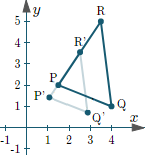
We can represent the point P(1.5, 2) as a column vector `[(\color(#f0f)1.5),(\color(#f0f)2)].`
Similarly, we can represent two points P(1.5, 2) and Q(4, 1) as a 2×2 vector `[(\color(#f0f)1.5, \color(#55f)4),(\color(#f0f)2, \color(#55f)1)].`
In most of the examples on this page, we have a triangle PQR, where R is (3.5, 5), and we represent the vertices of the triangle PQR as `[(\color(#f0f)1.5, \color(#55f)4, \color(#f55)3.5),(\color(#f0f)2, \color(#55f)1, \color(#f55)5)].` I've added color-coding so it's easier to see what's going on.
The linear transformation interactive applet
Things to do
- Read the description for the first transformation and observe the effect of multiplying the given matrix A on the original triangle PQR.
- Check the claim that multiplying by this particular A does actually produce the triangle P′Q′R′.
- When ready, click the "Next" button to move on to the next example.
Copyright © www.intmath.com
Summary of linear transformations
Reflection in the y-axis
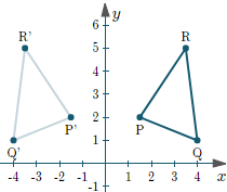
The general formula for reflection in the y-axis is:
`bb(Av)=[(-1,0),(0,1)][(x),(y)]`
`= [(-x),(y)]`
`=bb(v')`
Reflection in the x-axis
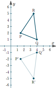
The general formula for reflection in the x-axis is:
`bb(Av)=[(1,0),(0,-1)][(x),(y)]`
`=[(x),(-y)]`
Reflection in the origin
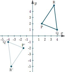
The general formula for reflection in the origin is:
`bb(Av)=[(-1,0),(0,-1)][(x),(y)]`
`=[(-x),(-y)]`
Rotation about the origin
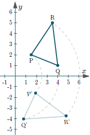
The general formula for rotation by angle θ about the origin is:
`bb(Av)=[(cos theta,sin theta),(-sin theta,cos theta)][(x),(y)]`
`= [(x cos theta + y sin theta),(-x sin theta + y cos theta)]`
Scaling
The general formula for scaling by an amount a in the x-direction and b in the y-direction is:
`bb(Av)=[(a, 0),(0, b)][(x),(y)]`
`=[(ax), (by)]`
Skewing (shearing) in the x- and y-directions
The general formula for skewing by an angle θ in the x-direction is:
`bb(Av)=[(1, -tan(theta)),(0, 1)][(x),(y)]`
`= [(x-ytan(theta)), (y)]`
The general formula for skewing by an angle θ in the y-direction is:
`bb(Av)=[(1, 0),(-tan(theta), 1)][(x),(y)]`
`= [(x), (y-xtan(theta))]`
Translation in the x- and y-directions
We cannot achieve translation using 2×2 matrices. So we need to extend both:
- Matrix A (to a 3×3 matrix) by adding a 3rd column containing the amount of translation we wish to achieve, and a 3rd "dumy" row of (0, 0, 1); and
- The vector v to a 3-row vector, by adding a "dummy" value 1.
The general formula for translating a point (x, y) by an amount a in the x-direction is:
`bb(Av)=[(1, 0, a),(0,1,0), (0,0,1)][(x),(y),(1)]`
`= [(x+a), (y), (1)]`
The general formula for translating a point (x, y) by an amount b in the y-direction is:
`bb(Av)=[(1, 0, 0),(0,1,b), (0,0,1)][(x),(y),(1)]`
`= [(x), (y+b), (1)]`
What are linear transformations?
In all the above examples, the transformations brought about by applying the various matrices A in each case are linear transformations. What does that mean?
In general, a transformation F is a linear transformation if for all vectors v1 and v2 in some vector space V, and some scalar c,
F(v1 + v2) = F(v1) + F(v2); and
F(cv1) = cF(v1)
Relating this to one of the examples we looked at in the interactive applet above, let's see what this definition means in plain English.
Condition 1. Sum of vectors: If we apply the transformation to the sum of two vectors, we get the same result if we apply the transformation to each vector separately, then add the results. So for example, in our skew example above, if we take the transformation matrix `bb(A)=[(1,-0.5),(0,1)]` and the vectors `bb(v)_1 = [ (2),(-2)]` and `bb(v)_2= [(2),(2)]` and add them first, we get:
`[(1,-0.5),(0,1)]([ (2),(-2)] + [(2),(2)]) =
[(1,-0.5),(0,1)][ (4),(0)] = [(4),(0)]`
Now, let's apply the transformation to each vector separately, then add them.
`[(1,-0.5),(0,1)][ (2),(-2)] + [(1,-0.5),(0,1)][(2),(2)] = [(3),(-2)] + [(1),(2)] = [(4),(0)]`
Condition 2. Scalar multiplication: The second condition just means if we multiply a vector by a scalar, then apply the transformation, we get the same result as applying the transformation first to the vector, then multiplying by that same scalar.
For example, we'll use `bb(v)_1 = [ (2),(-2)]` again, and the scalar c = 5. Multiplying by the scalar first, then applying the transform, we get:
`[(1,-0.5),(0,1)](5[ (2),(-2)]) = [(1,-0.5),(0,1)][ (10),(-10)] = [(15),(-10)]`
Next, we perform the transform first, then multiply by the scalar.
`5([(1,-0.5),(0,1)][ (2),(-2)]) = 5[(3),(-2)] = [(15),(-10)]`
We achieved the same result.
So the skew transform represented by the matrix `bb(A)=[(1,-0.5),(0,1)]` is a linear transformation.
Each of the above transformations is also a linear transformation.
NOTE 1: A "vector space" is a set on which the operations vector addition and scalar multiplication are defined, and where they satisfy commutative, associative, additive identity and inverses, distributive and unitary laws, as appropriate. See more detail here: Vector spaces.
NOTE 2: Another example of a linear transformation is the Laplace Transform, which we meet later in the calculus section.
Classes of linear transformations
Linear transformations are divided into the following types.
a. Rigid transformations (distance preserving)
Rigid transformations leave the shape, lengths and area of the original object unchanged. Rigid transformations are:
- Translation
- Rotation
b. Similarity transformations (angle preserving)
Similarity transformations preserve the angles of the original object, but not necessarily the size. Similarity transformations are:
- Translation
- Rotation
- Uniform scale (the same amount of scale in the x- and y-directions)
c. Affine transformations (parallel preserving)
Affine transformations preserve any parallel lines, but may change the shape and size. Affine transformations are:
- Translation
- Rotation
- Scale
- Skew (shear)
Notice Rigid transformations are a subset of Similarity transformations, which are in turn a subset of Affine transformations.
