14. Normal Probability Distributions

The Normal Probability Distribution is very common in the field of statistics. Whenever you measure things like people's height, weight, salary, opinions or votes, the graph of the results is very often a normal curve.

The Normal Distribution

On this page...

Properties of a normal distribution
Area under the normal curve
Standard normal distribution
Percentages of the area under standard normal curve
The z-Table
Application - stock market

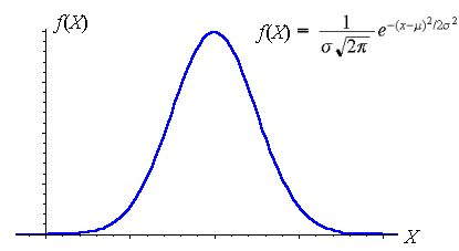
A random variable X whose distribution has the shape of a normal curve is called a normal random variable.

Normal Curve

This random variable X is said to be normally distributed with mean μ and standard deviation σ if its probability distribution is given by

$\qquad f(X)$ MATH

Properties of a Normal Distribution

The normal curve is symmetrical about the mean μ;
The mean is at the middle and divides the area into halves;
The total area under the curve is equal to 1;
It is completely determined by its mean and standard deviation σ (or variance σ²)

Note:

In a normal distribution, only 2 parameters are needed, namely μ and σ².

Area Under the Normal Curve using Integration

The probability of a continuous normal variable X found in a particular interval [a, b] is the area under the curve bounded by x = a and x = b and is given by

and the area depends upon the values of μ and σ.

[See Area under a Curve for more information on using integration to find areas under curves. Don't worry - we don't have to perform this integration - we'll use the computer to do it for us.]

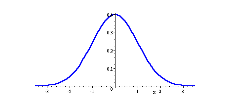
The Standard Normal Distribution

It makes life a lot easier for us if we standardize our normal curve, with a mean of zero and a standard deviation of 1 unit.

If we have the standardized situation of μ = 0 and σ = 1, then we have:

$\qquad f(X)$ MATH

Standard Normal Curve μ = 0, σ = 1

We can transform all the observations of any normal random variable X with mean μ and variance σ to a new set of observations of another normal random variable Z with mean 0 and variance 1 using the following transformation:

We can see this in the following example.

Example

Say μ = 2 and σ = 1/3 in a normal distribution.

The graph of the normal distribution is as follows:

μ = 2, σ = 1/3

The following graph represents the same information, but it has been standardized so that μ = 0 and σ = 1:

μ = 0, σ = 1

The two graphs have different μ and σ, but have the same shape (if we tweak the axes).

The new distribution of the normal random variable Z with mean 0 and variance 1 (or standard deviation 1) is called a standard normal distribution. Standardizing the distribution like this makes it much easier to calculate probabilities.

If we have mean μ and standard deviation σ, then

Since all the values of X falling between x₁ and x₂ have corresponding Z values between z₁ and z₂, it means:

The area under the X curve between X = x₁ and X = x₂ equals:

The area under the Z curve between Z = z₁ and Z = z₂.

Hence, we have the following equivalent probabilities:

P(x₁ < X < x₂) = P(z₁ < Z < z₂)

Example

Considering our example above where μ = 2, σ = 1/3, then

One-half standard deviation = σ/2 = 1/6, and

Two standard deviations = 2σ = 2/3

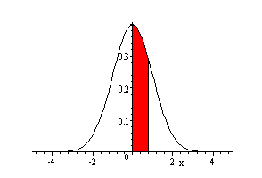
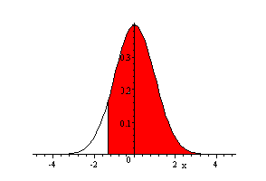
So $\dfrac{1}{2}$ s.d. to 2 s.d. to the right of μ = 2 will be represented by the area from $x_{1}=2\frac{1}{6}$ to $x_{2}=2\frac{2}{3}$ . This area is graphed as follows:

μ = 2, σ = 1/3

The area above is exactly the same as the area

z₁ = 0.5 to z₂ = 2

in the standard normal curve:

μ = 0, σ = 1

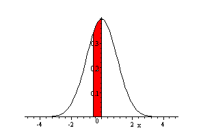
Percentages of the Area Under the Standard Normal Curve

A graph of this standardized (mean 0 and variance 1) normal curve is shown.

graph

In this graph, we have indicated the areas between the regions as follows:

-1 ≤ Z ≤ 1 68.27%

-2 ≤ Z ≤ 2 95.45%

-3 ≤ Z ≤ 3 99.73%

This means that 68.27% of the scores lie within 1 standard deviation of the mean.

This comes from: MATH

Also, 95.45% of the scores lie within 2 standard deviations of the mean.

This comes from: MATH

Finally, 99.73% of the scores lie within 3 standard deviations of the mean.

This comes from: MATH

The total area from -∞ < z < ∞ is 1.

The z-Table

The areas under the curve bounded by the ordinates z = 0 and any positive value of z are found in the z-Table. From this table the area under the standard normal curve between any two ordinates can be found by using the symmetry of the curve about z = 0. We can also use Scientific Notebook, as we shall see.

Go here for the actual z-Table.

EXAMPLE 1

Find the area under the standard normal curve for the following, using the z-table. Sketch each one.

(a) between z = 0 and z = 0.78

(b) between z = -0.56 and z = 0

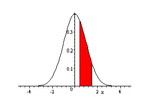
(d) between z = 0.44 and z = 1.50

(e) to the right of z = -1.33.

Answer

EXAMPLE 2

Find the following probabilities:

(a) P(Z > 1.06)

(b) P(Z < -2.15)

(d) P(-1.06 < Z < 4.00)

Answer

EXAMPLE 3

It was found that the mean length of 100 parts produced by a lathe was 20.05 mm with a standard deviation of 0.02 mm. Find the probability that a part selected at random would have a length

(a) between 20.03 mm and 20.08 mm

(b) between 20.06 mm and 20.07 mm

(d) greater than 20.09 mm.

Answer

EXAMPLE 4

A company pays its employees an average wage of $3.25 an hour with a standard deviation of 60 cents. If the wages are approximately normally distributed, determine

the proportion of the workers getting wages between $2.75 and $3.69 an hour;
the minimum wage of the highest 5%.

Answer

EXAMPLE 5

The average life of a certain type of motor is 10 years, with a standard deviation of 2 years. If the manufacturer is willing to replace only 3% of the motors that fail, how long a guarantee should he offer? Assume that the lives of the motors follow a normal distribution.

Answer

Application - The Stock Market

Sometimes, stock markets follow an uptrend (or downtrend) within 2 standard deviations of the mean. This is called moving within the linear regression channel.

Here is a chart of the Australian index (the All Ordinaries) from 2003 to Sep 2006.

asx

Image source: incrediblecharts.com.

The upper gray line is 2 standard deviations above the mean and the lower gray line is 2 standard deviations below the mean.

Notice in April 2006 that the index went above the upper edge of the channel and a correction followed (the market dropped).

But interestingly, the latter part of the chart shows that the index only went down as far as the bottom of the channel and then recovered to the mean, as you can see in the zoomed view below. Such analysis helps traders make money (or not lose money) when investing.