11. Probability Distributions - Concepts
On this page...
- Definitions of random, discrete and continuous variables
- Distribution function
- Probabilities as relative frequency
- Expected value
- Variance
- Standard deviation
Notation
We use upper case variables (like X and Z) to denote random variables, and lower-case letters (like x and z) to denote specific values of those variables.
Concept of Random Variable
The term "statistical experiment" is used to describe any process by which several chance observations are obtained.
All possible outcomes of an experiment comprise a set that is called the sample space. We are interested in some numerical description of the outcome.
For example, when we toss a coin `3` times, and we are interested in the number of heads that fall, then a numerical value of `0, 1, 2, 3` will be assigned to each sample point.
The numbers `0`, `1`, `2`, and `3` are random quantities determined by the outcome of an experiment.
They may be thought of as the values assumed by some random variable x, which in this case represents the number of heads when a coin is tossed 3 times.
So we could write x1 = 0, x2 = 1, x3 = 2 and x4 = 3.
Definitions
A random variable is a variable whose value is determined by the outcome of a random experiment.
A discrete random variable is one whose set of assumed values is countable (arises from counting).
A continuous random variable is one whose set of assumed values is uncountable (arises from measurement.).
We shall use:
A capital (upper case) X for the random variable and
Lower case x1, x2, x3... for the values of the random variable in an experiment. These xi then represent an event that is a subset of the sample space.
The probabilities of the events are given by: P(x1), P(x2), P(x3), ...
We also use the notation `P(X)`. For example, we may need to find some of the probabilities involved when we throw a die. We would write for the probability of obtaining a "5" when we roll a die as:
`P(X=5)=1/6`
Example 1 - Discrete Random Variable
Two balls are drawn at random in succession without replacement from an urn containing `4` red balls and `6` black balls.
Find the probabilities of all the possible outcomes.
Answer
Let X denote the number of red balls in the outcome.
| Possible Outcomes | RR | RB | BR | BB |
|---|---|---|---|---|
| X | 2 | 1 | 1 | 0 |
Here, x1 = 2, x2 = 1 , x3 = 1 , x4 = 0
Now, the probability of getting `2` red balls when we draw out the balls one at a time is:
Probability of first ball being red `= 4/10`
Probability of second ball being red `= 3/9` (because there are `3` red balls left in the urn, out of a total of `9` balls left.) So:
`P(x_1)=4/10times3/9=2/15`
Likewise, for the probability of red first is `4/10` followed by black is `6/9` (because there are `6` black balls still in the urn and `9` balls all together). So:
`P(x_2)=4/10times6/9 = 4/15`
Similarly for black then red:
`P(x_3)=6/10times4/9=4/15`
Finally, for `2` black balls:
`P(x_4)=6/10times5/9=1/3`
As a check, if we have found all the probabilities, then they should add up to `1`.
`2/15 + 4/15 + 4/15 + 1/3 = 15/15 = 1`
So we have found them all.
Example 2 - Continuous Random Variable
A jar of coffee is picked at random from a filling process in which an automatic machine is filling coffee jars each with `1\ "kg"` of coffee. Due to some faults in the automatic process, the weight of a jar could vary from jar to jar in the range `0.9\ "kg"` to `1.05\ "kg"`, excluding the latter.
Let X denote the weight of a jar of coffee selected. What is the range of X?
Answer
Possible outcomes: 0.9 ≤ X < 1.05
That's all there is to it!
Distribution Function
Definitions
-
A discrete probability distribution is a table (or a formula) listing all possible values that a discrete variable can take on, together with the associated probabilities.
- The function f(x) is called a probability density function for the continuous random variable X where the total area under the curve bounded by the x-axis is equal to `1`. i.e.
`int_(-oo)^oo f(x)dx=1`
The area under the curve between any two ordinates x = a and x = b is the probability that X lies between a and b.
`int_a^bf(x)dx=P(a<=X<=b)`
See area under a curve in the integration section for some background on this.
Probabilities As Relative Frequency
If an experiment is performed a sufficient number of times, then in the long run, the relative frequency of an event is called the probability of that event occurring.
Example 3
Refer to the previous example. The weight of a jar of coffee selected is a continuous random variable. The following table gives the weight in kg of `100` jars recently filled by the machine. It lists the observed values of the continuous random variable and their corresponding frequencies.
Find the probabilities for each weight category.
| Weight X | Number of Jars |
|---|---|
| `0.900 - 0.925` | `1` |
| `0.925 - 0.950` | `7` |
| `0.950 - 0.975` | `25` |
| `0.975 - 1.000` | `32` |
| `1.000 - 1.025` | `30` |
| `1.025 - 1.050` | `5` |
| Total | `100` |
Answer
We simply divide the number of jars in each weight category by 100 to give the probabilities.
| Weight X | Number of Jars |
Probability P(a ≤ X < b) |
|---|---|---|
| 0.900 - 0.925 | 1 | 0.01 |
| 0.925 - 0.950 | 7 | 0.07 |
| 0.950 - 0.975 | 25 | 0.25 |
| 0.975 - 1.000 | 32 | 0.32 |
| 1.000 - 1.025 | 30 | 0.30 |
| 1.025 - 1.050 | 5 | 0.05 |
| Total | 100 | 1.00 |
Expected Value of a Random Variable
Let X represent a discrete random variable with the probability distribution function P(X). Then the expected value of X denoted by E(X), or μ, is defined as:
E(X) = μ = Σ (xi × P(xi))
To calculate this, we multiply each possible value of the variable by its probability, then add the results.
Σ (xi × P(xi)) = { x1 × P(x1)} + { x2 × P(x2)} + { x3 × P(x3)} + ...
`E(X)` is also called the mean of the probability distribution.
Example 4
In Example 1 above, we had an experiment where we drew `2` balls from an urn containing `4` red and `6` black balls. What is the expected number of red balls?
Answer
We already worked out the probabilities before:
| Possible Outcome | RR | RB | BR | BB |
| xi | `2` | `1` | `1` | `0` |
| P(xi) | `2/15` | `4/15` | `4/15` | `1/3` |
`E(X)=sum{x_i * P(x_i)}`
`=2times2/15+` `1times4/15+` `1times4/15+` `0times1/3`
`=4/5`
`=0.8`
This means that if we performed this experiment 1000 times, we would expect to get 800 red balls.
Example 5
I throw a die and get `$1` if it is showing `1`, and get `$2` if it is showing `2`, and get `$3` if it is showing `3`, etc. What is the amount of money I can expect if I throw it `100` times?
Answer
For one throw, the expected value is:
`E(X)=sum{x_i*P(x_i)}=1times1/6+` `2times1/6+3times1/6+` `4times1/6+` `5times1/6+` `6times1/6`
`=7/2`
`=3.5`
So for 100 throws, I can expect to get $350.
Example 6
The number of persons X, in a Singapore family chosen at random has the following probability distribution:
| X | `1` | `2` | `3` | `4` | `5` | `6` | `7` | `8` |
|---|---|---|---|---|---|---|---|---|
| P(X) | `0.34` | `0.44` | `0.11` | `0.06` | `0.02` | `0.01` | `0.01` | `0.01` |
Find the average family size `E(X)`.
Answer
`E(X)`
`=sum{x_i*P(x_i)}`
`=1times0.34+2times0.44` `+3times0.11+4times0.06` `+5times0.02+6times0.01` `+7times0.01+8times0.01`
`=2.1`
So the average family size is E(X) = μ = 2.1 people.
Example 7
In a card game with my friend, I pay a certain amount of money each time I lose. I win `$4` if I draw a jack or a queen and I win `$5` if I draw a king or ace from an ordinary pack of `52` playing cards. If I draw other cards, I lose. What should I pay so that we come out even? (That is, the game is "fair"?)
Answer
| X | J, Q (`$4`) | K, A (`$5`) | lose (`-$x`) |
| P(X) | `8/52=2/13` | `2/13` | `9/13` |
`E(X)=sum{x_i * P(x_i)}`
`=4times2/13+5times2/13-xtimes9/13`
`=frac{18-9x}{13}`
Now the expected value should be $0 for the game to be fair.
So `frac{18-9x}{13}=0` and this gives `x=2`.
So I would need to pay `$2` for it to be a fair game.
Variance of a Random Variable
Let X represent a discrete random variable with probability distribution function `P(X)`. The variance of X denoted by `V(X)` or σ2 is defined as:
V(X) = σ2
= Σ[{X − E(X)}2 × P(X) ]
Since μ = E(X), (or the average value), we could also write this as:
V(X) = σ2
= Σ[{X − μ}2 × P(X) ]
Another way of calculating the variance is:
V(X) = σ2 = E(X2) − [E(X)]2
Standard Deviation of the Probability Distribution
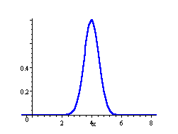
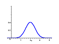
`sigma=sqrt(V(X)` is called the standard deviation of the probability distribution. The standard deviation is a number which describes the spread of the distribution. Small standard deviation means small spread, large standard deviation means large spread.
In the following 3 distributions, we have the same mean (μ = 4), but the standard deviation becomes bigger, meaning the spread of scores is greater.
The area under each curve is `1`.
Example 8
Find `V(X)` for the following probability distribution:
| X | `8` | `12` | `16` | `20` | `24` |
|---|---|---|---|---|---|
| P(X) | `1/8` | `1/6` | `3/8` | `1/4` | `1/12` |
Answer
We have to find `E(X)` first:
`E(X)` `=8times1/8+12times1/6` `+16times3/8+20times1/4` `+24times1/12` `=16`
Then:
`V(X)` `=sum[{X-E(X)}^2*P(X)]`
`=(8-16)^2 times 1/8 + (12-16)^2 times 1/6 ` `+ (16-16)^2 times 3/8 + (20-16)^2 times 1/4 ` `+ (24-16)^2 times1/12`
`=20`
Checking this using the other formula:
V(X) = E(X 2) − [E(X)]2
For this, we need to work out the expected value of the squares of the random variable X.
| X | `8` | `12` | `16` | `20` | `24` |
| X2 | `64` | `144` | `256` | `400` | `576` |
| P(X) | `1/8` | `1/6` | `3/8` | `1/4` | `1/12` |
`E(X^2)=sumX^2P(X)`
`=64times1/8+144times1/6+` `256times3/8+` `400times1/4+` `576times1/12`
`=276`
We found E(X) before: `E(X) = 16`
V(X) = E(X2) − [E(X)]2 = 276 − 162 = 20, as before.