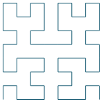
Animated Moore curve, a space-filling curve

Page by Murray Bourne, IntMath.com. Last updated: 13 February 2019.

The Moore Curve is an example of a space filling curve, continuous (one-dimensional) fractal lines that bend around in ever more intricate ways such that they eventually fill a (2-dimensional) square.

Below is an animation of one example of such curves, the Moore Curve, a variant of the Hilbert Curve first described by the German mathematician David Hilbert in 1891. At end of the 19th century, Italian mathematician Giuseppe Peano and David Hilbert worked on space-filling curves, an extension of the Cantor set.

Like many areas of experimental "pure" mathematics, there are several interesting real-world applications arising from this work, some of which are listed below the animation.

Note

Space-filling curves actually should be continuous, i.e. start at one point and finish at another point on the surface, not involve two "halves" meeting like in the animation below. This approach was chosen for the visual effect. (Yeah, I know it's not strictly correct.)

Things to do

This is a simple interactive. You can:

1. Just let it run (it will show the Moore curves for "path spacing" of 1, 1/3, 1/7, 1/15, 1/31, 1/63 of the square, successively) and observe how each new curve covers more of the square.
2. Choose one of the increments and it will start from there
3. Choose to make the line thicker, thus covering the square entirely.

Applications of space-filling curves

The concept behind "covering" a multi-dimensional object with a single-dimensional line has inspired researchers to improve computer efficiency in the following ways:

1. Indexing of data so database retrieval and manipulation is quicker, which improves search capabilities
2. Disk scheduling (where and when to store and retrieve data)
3. Spatial access methods
4. Clustering
5. Image compression

John J. Bartholdi III, Professor of Industrial and Systems Engineering, in Some combinatorial applications of spacefilling curves also applied the space-filling curve concept to the famous travelling salesman problem (where a salesman needs to cover all the cities in an area, for the shortest cost, time or distance) in the following ways:

1. To build a routing system for Meals-on-Wheels in Fulton County (Atlanta, GA)
2. To route blood delivery by the American Red Cross to hospitals in the Atlanta metropolitan area.
3. To target a space-based laser for the Strategic Defense Iniative (commonly known as the "Star Wars" program).
4. To control a pen-plotter for the drawing of maps.

Further reading: A Routing System Based On Spacefilling Curves

See also this article from the journal Nature which includes an interesting application of space-filling curves to energy storage devices: Bioinspired fractal electrodes for solar energy storages

The math behind the animation

The math behind the coding of this space-filling curve involved:

1. Transformational geometry: translations and rotations
2. Trigonometry: sine and cosine of angles to produce segments pointing in the correct direction
3. Arrays: to direct and keep track of the segments

The code

I originally thought this would be quite quick to code, since the following Moore Curve algorithm was given in several sources:

Alphabet: L, R
Constants: F, +, −
Axiom: LFL+F+LFL
Production rules:
L → −RF+LFL+FR−
R → +LF−RFR−FL+
Here, F means "draw forward", + means "turn left 90°", and − means "turn right 90°"

I expected I would need to set up this generic set of directions up for the first curve, and then simply apply it for subsequent curves. However, that was not how it transpired and it turned out to be much more involved.

After trying several different approaches, I ended up proceeding as follows:

1. The first 3 curves are treated separately (it was a nightmare to try to generalize the approach for these simpler cases).
2. The curves 1/15 through 1/63 involve creating this basic shape (which is the Hilbert Curve) as an SVG path.
   
3. Next we animate the drawing of the curve (strating in the lower right-hand corner) using the stroke-dashoffset approach, which I've used before to produce efficient curve animations as seen in e.g. Graphs of Sine and Cosine (The following are animated GIFs, so they are not as smooth as the SVG originals)
   
4. Often, the animation had to go in reverse so that it joined correctly and went in the right direction. I achieved that by reversing the points in the SVG path node and animating as before. This gave us:
   
5. Then I had to rotate them by an appropriate multiple of 90°
6. Next, they needed to be placed in the correct positions.
7. Finally, once the animation had finished, the block was replaced by a copy of the fixed version, then we moved on to the next block position and repeated the process.

Credits

The curves are based on the ones given in Wikipedia's Moore Curve page.