6. Composite Trigonometric Curves
by M. Bourne
a. Adding trigonometric and other functions
When adding 2 or more trigonometric graphs, we add ordinates (y-values) to find the resultant curve.
Later, on this page...
Example 1: Electronics
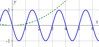
One of the simplest examples of composite trigonometric curves is from electronics. An AC (alternating current) signal (v = 3 cos 8t) is added to a `10` volt DC (direct current) voltage source. The resulting signal looks like the following.
Graph of `v=10+3cos 8t`, the sum of a DC and an AC voltage.
The combined graph that you see has equation: v = 10 + 3 cos 8t.
We are simply adding `10` to all the v-values of the cosine curve.
Water waves
Example 2
When two water waves meet on a pond, they combine such that when 2 crests meet, they are added to give a larger crest, and when 2 troughs meet, they add to give a deeper trough. A crest and a trough tend to cancel each other out when they meet.
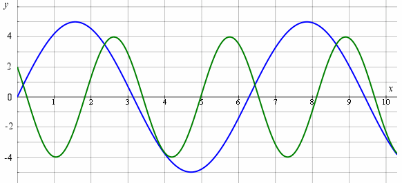
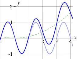
In this example, let's assume the following 2 waves meet.
`a(x) = 5 sin x`
`b(x) = 4 cos(2x + π/3) `
Sketch the graph of the combined wave:
`y=5 sin(x)+4 cos(2x+pi/3)`
Answer
Of course, we could make a table of values and substitute millions of values of x and join the dots. But this is very dangerous because we don't have a sense of what is going on and our joined dots will look like unrelated spaghetti.
It is best to first sketch the graphs of the 2 parts of this function on the same graph.
`a(x) = 5\ sin\ x` (in blue)
`b(x) = 4\ cos(2x + π/3) ` (in green)
Now, we need to add the ordinates ( y-values) of each part to obtain the composite graph. Let's take a few values.
When x = 0,
`a(0) = 5\ sin\ 0 = 0`
`b(0) = 4\ cos(π/3) = 2`
Adding these,
a(0) +b(0) = 0 + 2 = 2
Likewise, when x = 1 (radians, of course),
`a(1) = 5\ sin\ 1 = 4. 21`
`b(1) = 4\ cos(2 + π/3) = -3. 98`
Adding gives:
a(1) + b(1) = 0.23
Similarly, for x = 2, a(2) + b(2) = 5.86
x = 3: a(3) + b(3) = 3.59
x = 4: a(4) + b(4) = -7.50
x = 5: a(5) + b(5) = -4.59
Here is the result of adding the 2 separate waves together.
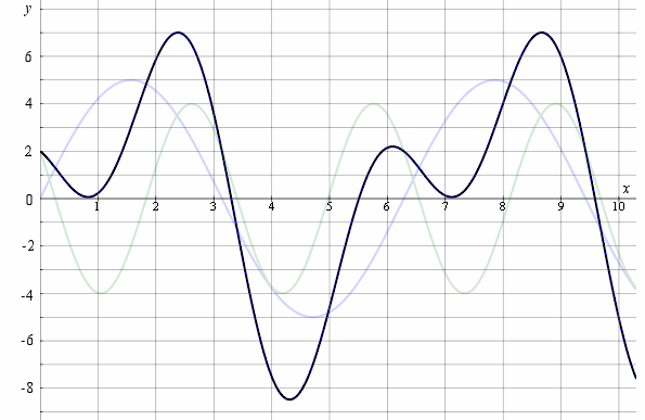
Notice the two crests near `x = 2.5` have added together to give a large crest (around 7). The two troughs near `x = 4.5` have added together to give a deep trough.
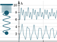
Example 3: Double springs interactive graph
We have two springs with different thicknesses (and spring constants) with two different sized masses connected and hanging vertically. While holding the top mass still, we pull down the bottom mass. Then we let go of both masses and allow the system to move freely.
We can also grab the mass in the middle to compress or stretch the top spring.
In a real experiment, we'd have a motion sensor connected to a computer and we would be able to see the resulting movement of the masses as time progresses, just as you can in this simulation.
(You need to "reset" the whole thing to drag the masses again.)
Copyright © www.intmath.com Frame rate: 0
Stretch (or compress) either of the springs by dragging either of the masses, then let go to see the resulting waveforms. Such waveforms are the result of adding different trigonometric curves.
Notes:
- Our springs are constrained to move in one dimension only.
- The springs slow down as time goes on, due to friction.
- You can see other spring examples in Graphs of y = a sin bx and y = a cos bx, and in the section on Work by a Variable Force, which is an application of Calculus.
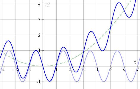
Depending on the masses, the lengths of the springs and the spring constants, we could get a curve similar to the following (for one or the other mass positions), which is the sum of two cosine curves:
x = 0.0572 cos(4.667t) + 0.0218 cos(12.22t)
Graph of `x=0.0572 cos(4.667t) + 0.0218 cos(12.22t)`, a composite trigonometric model of a double spring system.
[The function x(t) given above is obtained using differential equations, an interesting topic which we meet later in the calculus section.]
Need Graph Paper?

Reference: Morland, T "Modeling a Simple Mechanical System", Teaching Mathematics and Its Applications, Vol 18 No 2 1999.
Exercises
1. Graph the composite trigonometric curve `y = x^2/10 − sin\ πx`
Answer
We recognise `y=x^2/10` as a parabola, that we met before.
We draw the two curves `y=x^2/10` (green, dotted) and `y = -sin\ πx` (blue) on the same set of axes.
The sum of the y-ordinates of the two curves is shown next:
Expanding the domain (that is, zooming out) gives us a better view of the parabola added to the sine curve:
2. Graph the curve y = 2 cos 2x + 3 sin x
Answer
We have plotted y = 2 cos 2x (light blue) and y = 3 sin x (dotted light green) so you can see where the composite graph comes from.
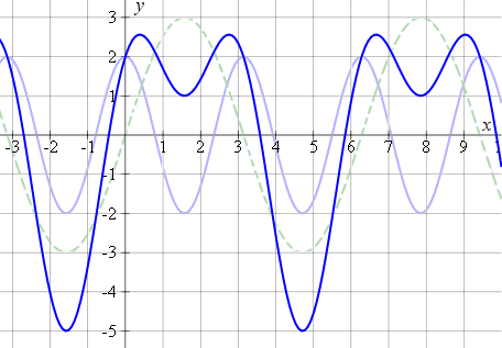
Note 1: You will notice in this last example that there is a regular pattern forming. In fact, it is a simple example of a Fourier Series, which we meet (much) later in the Advanced Calculus section.
Note 2: Of course, we will mostly use the computer to graph these composite graphs. It is often very tedious to add many y-values in a table. However, the important thing is to understand that a composite graph is the sum of the y-values of two (or more) graphs. Or, we can have products (and quotients) of functions that will also give us composite trigonometric graphs.
Example 4: Real-world Case
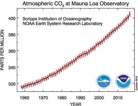
Atmospheric carbon dioxide levels have been rapidly increasing since the beginning of the industrial revolution.
This chart using data from the National Oceanographic and Atmospheric Administration shows the increase in CO2 since records began in 1958, on Mauna Loa in Hawaii. The dark green line is yearly averages, while the magenta (pink) line gives weekly readings (the data start in 1974), that go up and down with the seasons.
Atmospheric CO2 at Mauna Loa Observatory
CO2 concentrations - weekly data with yearly averages.
[Latest data: 08 Sep 2024]
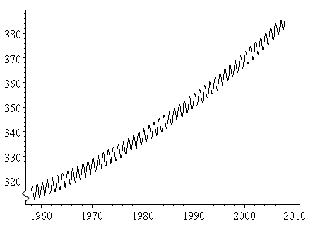
We can closely model the (pink) weekly curve as the sum of a cosine and cubic curve as follows:
y = 3.5 cos(2πx − 1.2) + 0.00002052590807(x − 1958)3 + 0.01105601542(x − 1958)2 + 0.8044611048(x − 1958) + 314.634017
(For more background and information on where this model came from, see Earth killer - composite trigonometry CO2 graph.)
Here is the graph of the model. It is similar to what we had in Exercise 1 above.
Example 5: Standing wave
We have two sine curves with the same period and amplitude, moving left to right (they gray curve) and right to left (the magenta curve). The sum of those two curves is a standing wave, one that doesn't move left-right, but is stationary, and at its full extent, has twice the amplitude of the gray and magenta sine curves.
Copyright © www.intmath.com Frame rate: 0
The dots along the x-axis are called nodes, where there is no movement of the particles making up the waves.
b. Composite Trigonometric Graphs - Product of Functions
The following examples show composite trigonometric graphs where we are taking the product of two functions.
Example 6: Graph the function y = x sin x
In this example, we are multiplying the sine of each x-value by the x-value.
So for example, if `x = 2`, the y-value will be `y = 2 sin 2 = 1.819`.
Answer
Graph of `y = x sin x`, a composite trigonometric curve involving product of functions.
The crests and troughs extend to the lines y = x and y = −x (the grey dashed lines).
Notice that the amplitude continually increases. The energy in this wave becomes greater as we move further along the x-axis.
Example 7: RCL Circuit - Constant Forced Response
In electronics, an RCL circuit has a resistor, a capacitor and an inductor connected in series. If we apply a constant voltage to the circuit, there is an initial pulse in the current. The resulting function is a product of an exponential decay function and a sin function.
i = e-0.3t sin t
The graph of the current at time t has the following appearance. The current reduces quickly after the initial pulse.
Graph of `i=e^(-0.3t)sin(t)`, a composite trigonometric curve of an RLC circuit response.
We learn how to solve these problems later in Applications of Second Order Differential Equations.