2. Full Range Fourier Series
The Fourier Series is an infinite series expansion involving trigonometric functions.
A periodic waveform f(t) of period p = 2L has a Fourier Series given by:
`f(t)` `=(a_0)/2 + sum_(n=1)^ooa_ncos((npit)/L)` `+sum_(n=1)^oo b_n\ sin((npit)/L)`
`=(a_0)/2+a_1cos((pit)/L)` `+a_2cos((2pit)/L)` `+a_3cos((3pit)/L)+...` `+b_1sin((pit)/L)` `+b_2sin((2pit)/L)` `+b_3sin((3pit)/L)+...`
Helpful Revision
where
an and bn are the Fourier coefficients,
and
`(a_0)/2` is the mean value, sometimes referred to as the dc level.
Fourier Coefficients For Full Range Series Over Any Range -L TO L
If `f(t)` is expanded in the range `-L` to `L` (period `= 2L`) so that the range of integration is `2L`, i.e. half the range of integration is `L`, then the Fourier coefficients are given by
`a_0=1/Lint_(-L)^Lf(t)dt`
`a_n=1/Lint_(-L)^Lf(t)"cos"(npit)/Ldt`
`b_n=1/Lint_(-L)^Lf(t)\ "sin"(npit)/Ldt`
where `n = 1, 2, 3 ...`
NOTE: Some textbooks use
`a_0=1/(2L)int_(-L)^Lf(t)dt`
and then modify the series appropriately. It gives us the same final result.
Dirichlet Conditions
Any periodic waveform of period `p = 2L`, can be expressed in a Fourier series provided that
(a) it has a finite number of discontinuities within the period `2L`;
(b) it has a finite average value in the period `2L`;
(c) it has a finite number of positive and negative maxima and minima.
When these conditions, called the Dirichlet conditions, are satisfied, the Fourier series for the function `f(t)` exists.
Each of the examples in this chapter obey the Dirichlet Conditions and so the Fourier Series exists.
Example 1: Fourier Series - Square Wave
Sketch the function for 3 cycles:
`f(t)={(0, if -4<=t<0),(5, if 0<=t<4):}`
`f(t) = f(t + 8)`
Find the Fourier series for the function.
Interactive: You can explore this example using this interactive Fourier Series graph.
Solution:
Here's one possible way to solve it:
Answer
The sketch of the function:
Graph of `f(t)`, a rectangular function.
We need to find the Fourier coefficients a0, an and bn before we can determine the series.
`a_0=1/Lint_(-L)^Lf(t)dt`
`=1/4int_(-4)^4f(t)dt`
`=1/4(int_(-4)^0(0)dt+int_0^4(5)dt)`
`=1/4(0+[5t]_0^4)`
`=1/4(20)`
`=5`
Note 1: We could have found this value easily by observing that the graph is totally above the t-axis and finding the area under the curve from t = −4 to t = 4. It is just 2 rectangles, one with height `0` so the area is `0`, and the other rectangle has dimensions `4` by `5`, thus the area is `20`. So the integral part has value `20`; and `1/4` of `20 = 5`.
Note 2: The mean value of our function is given by `(a_0)/2`. Our function has value 5 for half of the time and value 0 for the other half, so the value of `(a_0)/2` must be 2.5. So a0 will have value 5.
These points can help us check our work and help us understand what is going on. However, it is good to see how the integration works for a split function like this.
`a_n=1/Lint_(-L)^L f(t)\ cos {:(n pi t)/L:} dt`
`=1/4int_(-4)^4f(t)\ cos {:(n pi t)/4 :}dt`
`=1/4(int_(-4)^0(0) cos {:(n pi t)/4 :} dt:}` `{: + int_0^4(5) cos {:(n pi t)/4 :}dt)`
`=1/4(0+[5 4/(n pi) sin {:(n pi t)/4 :}]_0^4)`
`=1/4xx5xx4/(n pi)([sin {: (n pi t)/4 :}]_0^4)`
`=5/(n pi)( sin {: (n pi (4) )/4 :} - sin {: (n pi (0) )/4 :} )`
`=5/(n pi)(sin n pi-0)`
`=0`
Note 3: In the next section, Even and Odd Functions, we'll see that we don't even need to calculate an in this example. We can tell it will have value 0 before we start.
`b_n=1/Lint_(-L)^Lf(t)\ sin {:(n pi t)/L:}dt`
`=1/4int_(-4)^4f(t)\ sin {:(n pi t)/4:}dt`
`=1/4(int_(-4)^0(0)\ sin {:(n pi t)/4 :}dt` `{:+int_0^4(5)\ sin {:(n pi t)/4 :}dt)`
`=1/4(0:}` `{:+[(-5) (4/(n pi)) cos {:(n pi t)/4:}]_0^4)`
`=-(1/4)(5)(4/(n pi))[cos {:(n pi t)/4 :}]_0^4`
`=-5/(n pi)(cos {:(n pi(4))/4:}-1)`
`=-5/(n pi)(cos n pi-1)`
At this point, we can substitute this into our Fourier Series formula:
`f(t)=a_0/2+sum_(n=1)^oo a_n\ cos {:(n pi t)/L :}` `+sum_(n=1)^oo b_n\ sin {:(n pi t)/L:}`
`=5/2+sum_(n=1)^oo(0)\ cos {:(n pi t)/4 :}` `+sum_(n=1)^oo-5/(n pi)(cos n pi-1)\ sin {:(n pi t)/4:}`
`=2.5` `-5/pisum_(n=1)^oo1/n(cos npi-1)\ sin {:(n pi t)/4:}`
Now, we substitute `n = 1, 2, 3,...` into the expression inside the series:
`n` `1/n(cos npi-1)sin{:(n pi t)/4 :}` `1` `1/1(cos pi-1)\ sin{:(pi t)/4 :}` `=-2\ sin {:(pi t)/4 :}` `2` `1/2(cos 2pi-1)\ sin{:(2 pi t)/4 :}=0` `3` `1/3(cos 3pi-1)\ sin{:(3pi t)/4 :}` `=-2/3\ sin {:(3pi t)/4 :}` `4` `1/4(cos 4pi-1)\ sin{:(4 pi t)/4 :}=0` `5` `1/5(cos 5pi-1)\ sin{:(5 pi t)/4 :}` `=-2/5\ sin {:(5 pi t)/4 :}` `6` `1/6(cos 6pi-1)\ sin{:(6 pi t)/4 :}=0` `7` `1/7(cos 7pi-1)\ sin{:(7pi t)/4 :}` `=-2/7\ sin {:(7 pi t)/4 :}`
Now we can write out the first few terms of the required Fourier Series:
`f(t)=2.5-5/pi(-2\ sin{:(pi t)/4:}` `-2/3 sin {:(3pit)/4:}` `{:-2/5 sin {:(5pit)/4:}-...)`
`=2.5+10/pi(sin {:(pi t)/4:}` `+1/3 sin {:(3 pit)/4:}` `+1/5 sin {:(5pi t)/4:}` `{:+...)`
Alternative approach:
Answer
Alternatively, we could observe that every even term is 0, so we only need to generate odd terms. We could have expressed the `b_n` term as:
`b_n=-5/(n pi)(cos n pi-1)`
`=-5/(n pi)((-1)^n-1)`
`=10/(n pi)`, if `n` is odd, and `0` if `n` is even.
To generate odd numbers for our series, we need to use:
`b_n=10/((2n-1)pi),\ \ \ n=1,2,3...`
We also need to generate only odd numbers for the sine terms in the series, since the even ones will be 0.
So the required series this time is:
`f(t)=a_0/2` `+sum_(n=1)^oo a_n\ cos {:(n pi t)/L :}` `+sum_(n=1)^oob_n\ sin {:(n pi t)/L:}`
`=5/2` `+sum_(n=1)^oo(0)\ cos {:(n pi t)/4:}` `+sum_(n=1)^oo 10/((2n-1)pi) sin {:((2n-1)pi t)/4:}`
`=2.5` `+10/pi sum_(n=1)^oo 1/((2n-1)) sin {:((2n-1)pi t)/4:}`
The first four terms series are once again:
`f(t)=2.5+10/pi(sin {:(pi t)/4:}` `+1/3 sin {:(3 pit)/4:}` `+1/5 sin {:(5pi t)/4:}` `{:+1/7 sin {:(7pi t)/4:}...)`
[NOTE: Whichever method we choose, n must take values `1, 2, 3, ...` when we are writing out the series using sigma notation.]
What have we done?
Let's think about what the answer in the above example means.
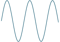
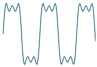
We are adding a series of sine terms (with decreasing amplitudes and decreasing periods) together. The combined signal, as we take more and more terms, starts to look like our original square wave:
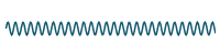
We start with this sine curve:
`2.5+10/pi sin((pi t)/4)`
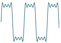
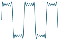
We then add the y-values of the second sine curve (with lower amplitude and higher frequency) to the above curve, and get the following:
Original graph
+
`10/(3pi)sin((3 pi t) /4)`
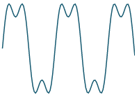
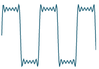
We continue as follows:
Previous result
plus
`10/(5pi)sin((5 pi t) /4)`
Previous result
plus
`10/(7pi)sin((7 pi t)/4)`
Previous result
plus
`10/(9pi)sin((9 pi t)/4)`
Previous result
plus
`10/(11pi)sin((11 pi t)/4)`
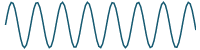
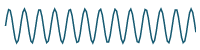
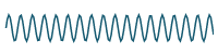
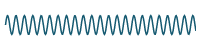
If we graph the result of adding more and more terms, we can see that our series will closely approximate the original periodic function. We graph the first 20 terms and see we are getting "very close" to the original function.:
`2.5+10/pi sum_(n=1)^20 1/((2n-1))"sin"((2n-1)pit)/4`
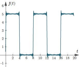
Apart from helping us understand what is going on, a graph can help us check our calculations.
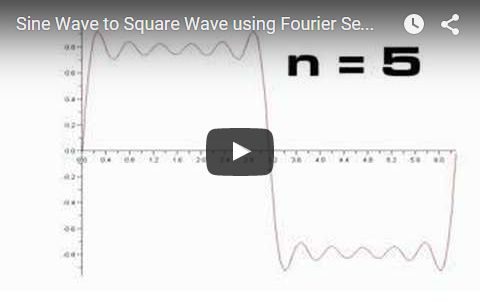
The following video illustrates what we are doing. The equation is not exactly the same, but the concept is. The tone heard at the end is (close to) a "pure" square wave.
Common Case: Period = 2L = 2π
If a function is defined in the range -π to π (i.e. period 2L = 2π radians), the range of integration is 2π and half the range is L = π.
The Fourier coefficients of the Fourier series f(t) in this case become:
`a_0=1/piint_(-pi)^pif(t)dt`
`a_n=1/piint_(-pi)^pif(t)\ cos nt\ dt`
`b_n=1/piint_(-pi)^pif(t)\ sin nt\ dt`
and the formula for the Fourier Series becomes:
`f(t)` `=a_0/2+sum_(n=1)^oo\ a_n\ cos nt` `+sum_(n=1)^oo\ b_n\ sin nt`
where `n = 1, 2, 3, ...`
Example 2
a) Sketch the waveform of the periodic function defined as:
`f(t) = t\ \ if\ \ -π < t < π`
`f(t) = f(t + 2π)` for all `t`.
b) Obtain the Fourier series of `f(t)` and write the first 4 terms of the series.
Answer
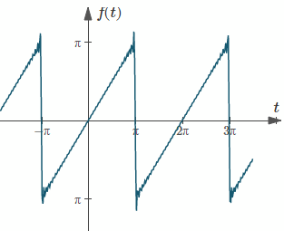
a) Sketch:
Graph of `f(t)`, a sawtooth curve.
b) First, we need to find the Fourier coefficients `a_0`, `a_n` and `a_b`.
`a_0=1/piint_(-pi)^pif(t)dt`
`=1/piint_(-pi)^pit\ dt`
`=1/pi[t^2/2]_-pi^pi`
`=1/pi[{:pi:}^2/2-{:pi:}^2/2]`
`=0`
Next, we use a result from the Table of Integrals:
`intt\ cos nt\ dt` `=1/n^2(cos nt + nt\ sin nt)`
We have:
`a_n=1/pi int_(-pi)^pif(t)cos nt\ dt`
`=1/pi int_(-pi)^pit\ cos nt\ dt`
`=1/pi[1/n^2(cos nt+nt\ sin nt)]_(-pi)^pi`
`=1/(pin^2)[(cos n pi+0)` `{:-(cos(-n pi)+0)]`
`=1/(pi n^2)(cos n pi-cos n pi)`
`=0`
To find `b_n`, once again we use a result from our Table of Integrals
`intt\ sin nt\ dt` `=1/n^2(sin nt-nt\ cos nt)`
We have:
`b_n=1/piint_(-pi)^pif(t)\ sin nt\ dt`
`=1/piint_(-pi)^pit\ sin nt\ dt`
`=1/pi[1/n^2(sin nt-nt\ cos nt)]_(-pi)^pi`
`=1/(n^2pi)([0-n pi\ cos n pi]` `{:-[0+n pi\ cos(-n pi)])`
`=(n pi)/(n^2pi)(-2\ cos n pi)`
`=-2/ncos npi`
`=-2/n(-1)^n`
`=2/n(-1)^(n+1)`
Now to put it all together for the Fourier Series for our function:
`f(t)=a_0/2` `+sum_(n=1)^oo(a_n\ cos nt` `{:+b_n\ sin nt)`
`=0/2` `+sum_(n=1)^oo((0)\ cos nt` `{:+2/n(-1)^(n+1)sin nt)`
`=sum_(n=1)^oo(2/n(-1)^(n+1)sin nt)`
`=2\ sin t` `-sin 2t` `+2/3sin 3t-1/2sin 4t+...`
What have we found?
The graph of the first 40 terms is:
`f(t) ~~ sum_(n=1)^40(2/n(-1)^(n+1)\ sin nt)`
Interactive: You can explore this example using this interactive Fourier Series graph.
Expressing Fourier Series in other Forms
We can express the Fourier Series in different ways for convenience, depending on the situation.
Fourier Series Expanded In Time t with period T
Let the function f(t) be periodic with period `T = 2L` where
`omega=(2pi)/T=(2pi)/(2L)=pi/L`
In this case, our lower limit of integration is `0`.
Hence the Fourier series is
`f(t)=a_0/2+sum_(n=1)^oo\ a_n\ cos n omega t` `+sum_(n=1)^oo\ b_n\ sin n omega t`
where
`a_0=omega/piint_0^(2pi//omega)f(t)dt`
`a_n=omega/piint_0^(2pi//omega)f(t)\ cos n omega t\ dt`
`b_n=omega/piint_0^(2pi//omega)f(t)\ sin n omega t\ dt`
(Note: half the range of integration `pi/omega`.)
Fourier Series Expanded in Angular Displacement ω
(Note: ω is measured in radians here)
Let the function `f(ω)` be periodic with period `2L`.
We let ` θ = ωt`. This function can be represented as
`f(theta)` `=a_0/2` `+sum_(n=1)^oo(a_n\ cos (n pi theta)/L:}` `{:+\ b_n\ "sin" (n pi theta)/L)`
where
`a_0=1/Lint_0^(2L)f(theta)d theta`
`a_n=1/Lint_0^(2L)f(theta)\ cos"(n pi theta)/Ld theta`
`b_n=1/Lint_0^(2L)f(theta)\ sin"(n pi theta)/Ld theta`